2-DOF Inverse Kinematics

This example demonstrates how to use inverse kinematics (IK) for a flapping wing system with two rotational degrees of freedom (DoF).

Using FlapKine, the goal is to calculate the Euler angles required to reproduce a desired wing motion. The target motion is first captured using a multi-view stereo camera setup, which provides accurate 3D wing positions.

Note

Multi-view stereo processing is not currently built into FlapKine, but future versions aim to include native support for it.

At present, we use DLTdv [1] to process video recordings and generate 3D positional data. FlapKine then takes this data as input and computes a time series of Euler angles needed to recreate the wing motion through inverse kinematics.

This workflow highlights how FlapKine serves as a powerful tool for post-processing and analyzing real-world motion capture data using analytical IK models.

Overview

In this example, the wing structure undergoes:

• Rotation about two orthogonal axes: the z-axis and the x-axis.

To compute the Euler rotation angles, we select two pairs of points on the wing:

• Two points along the wing span to define the body-frame x-axis.

• Two points along the wing chord to establish the orientation in 3D space.

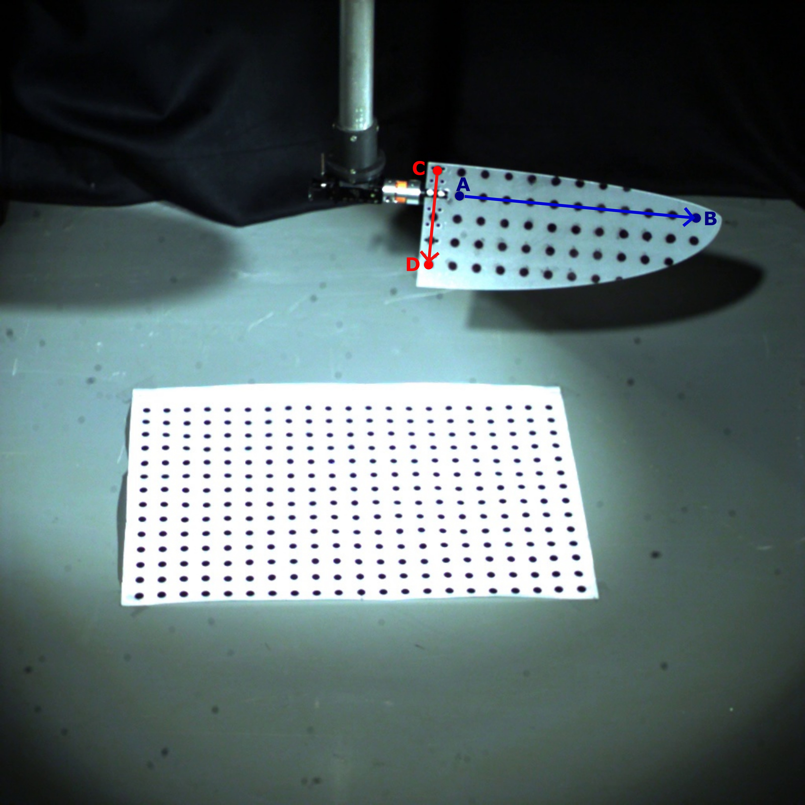
These specific points (A, B, C, D) are marked on the wing as shown in the image below. They are manually tracked frame-by-frame using DLTdv.

After tracking, the 2D point data is converted into 3D coordinates using DLTdv’s calibration. The result is stored in a frame-wise format as shown below:

pt1_x, pt1_y, pt1_z, pt2_x, pt2_y, pt2_z, pt3_x, pt3_y, pt3_z, pt4_x, pt4_y, pt4_z
1.23, 4.56, 7.89, 2.34, 5.67, 8.90, 3.45, 6.78, 9.01, 4.56, 7.89, 0.12
1.25, 4.58, 7.91, 2.36, 5.69, 8.92, 3.47, 6.80, 9.03, 4.58, 7.91, 0.14
...

• pt1_x, pt1_y, pt1_z: X, Y, Z coordinates of point A

• pt2_x, pt2_y, pt2_z: X, Y, Z coordinates of point B

• pt3_x, pt3_y, pt3_z: X, Y, Z coordinates of point C

• pt4_x, pt4_y, pt4_z: X, Y, Z coordinates of point D

These markers correspond to the labeled points in the image below, used to define body orientation and compute IK-based Euler angles.

Files Included

• `project.zip`: A compressed archive containing the full simulation setup and all necessary resource files.

After extracting, the contents are organized into the following directories:

• `2_DOF_INV/` – Contains the FlapKine project configuration and execution setup.

• `resources/` – Includes supporting assets such as STL meshes, camera videos, calibration data, and tracked 3D coordinates.

Project Folder Structure

The 2_DOF_INV/ directory contains the core FlapKine project files:

2_DOF_INV/
├── scene.pkl          # Serialized Scene object containing the simulation setup
├── config.json        # Configuration file for rendering and simulation parameters
└── data/              # Directory where output frames and videos are generated

Resource Files

The resources/ directory contains all the data used to reconstruct and analyze the wing motion:

resources/
├── videos/
│   ├── view_1.mp4                  # Wing motion video from camera 1
│   └── view_2.mp4                  # Wing motion video from camera 2
│
├── camera_calibration/
│   ├── calibration_cube/
│   │   ├── view_1.jpg              # Image of calibration object from camera 1
│   │   ├── view_2.jpg              # Image of calibration object from camera 2
│   │   └── cube_dimensions.jpg     # Reference image showing cube dimensions
│   └── calibration_matrix.csv      # Computed stereo calibration matrix
│
├── stl/
│   └── wing.stl                    # 3D mesh of the wing model
│
└── dlt_results/
    └── 3d_positions.csv            # Tracked 3D coordinates of wing markers (A–D)

Initial STL Orientation

The wing.stl model is oriented such that:

• The x-axis aligns with the wing span.

• The y-axis aligns with the wing chord.

• The z-axis corresponds to the wing thickness.

Running the Example

1. Extract the project.zip archive to your desired directory.

2. Launch FlapKine and select Load Project.

3. Navigate to the 2_DOF_INV/ folder and open the project.

4. The project will load with the pre-configured scene.

5. To visualize the simulation, click on the Render button. The output video will be saved under data/videos/.

   Note

   For detailed information on the GUI functionalities, refer to the Project Editor Window section.

Below is a preview of the rendered simulation output:

Figure: Rendered simulation preview after executing the inverse kinematics setup in FlapKine.

For higher quality or longer playback, you can render a full-resolution .mp4 video directly using the Render button. The video will be saved automatically in the data/videos/ folder within your project directory.

Reproducing from Scratch

To manually recreate the above project from scratch:

1. Open FlapKine and select New Project.

2. Choose your desired destination folder, enter a project name, and click Save.

3. The Project Creator Window will open. This is where you can import Scene and change rendering configurations.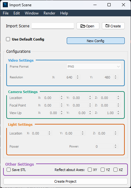

   

   Figure: Screenshot of the project creator window in FlapKine.

4. Start by loading the default rendering configuration:

   • Toggle the Use Default Config option.

   • You may change the configuration settings according to your desire. However default config works with this project.

   • Disable Reflect

   

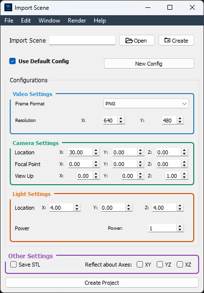
   Figure: Rendering configuration settings in FlapKine.

5. To add a model to the scene, click the Create button under the Import Scene section. This opens the Scene Creator Window.

   

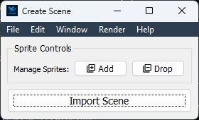
   Figure: Scene creator window in FlapKine.

6. Click Add to insert a new Sprite.

7. In the Sprite 1 section, click Create. This opens the Sprite Creator Window.

8. In the Sprite Creator:

   • Assign a name to your 3DObject.

   • Load the STL file from the resource/stl directory.

   

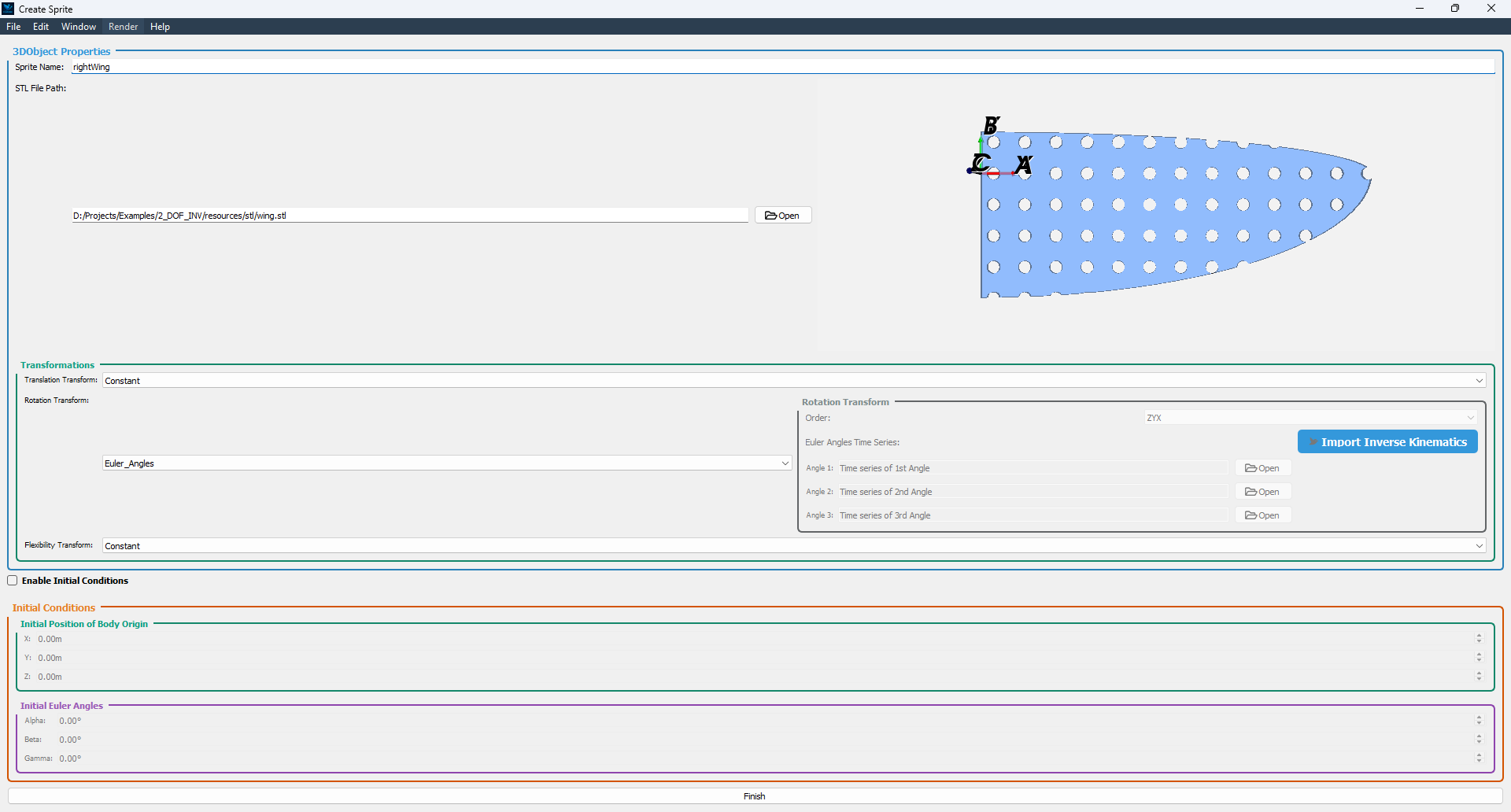
   Figure: STL file loaded and Transformation set in the sprite configuration.

9. In the Transformation section:

   • Set the Rotation Transform Type to Euler_angles.

   • Click the blue-colored Inverse Kinematics button to open the Inverse Kinematics Window.

   • In the Inverse Kinematics Window, press the Import Data button and select the dataset located in the resources/dlt_results/ directory.

   • Alternatively, you may compute the 3D positions independently using external software such as DLTdv, based on the provided video files.

   • However, for convenience, the required data has been pre-generated and included with the project to streamline the workflow.

   • After selecting the data, set the rotation order to XYZ. This will yield correctly calculated Euler angles. The time series of these angles will be displayed in the right-hand panel.

   • The left-hand panel provides a 3D visualization of the trajectories for each of the four tracked points: A, B, C, and D.

   • Once the analysis is complete, click the Finish button.

   • The computed Euler angle time series will then be automatically transferred to the Sprite Creator Window.

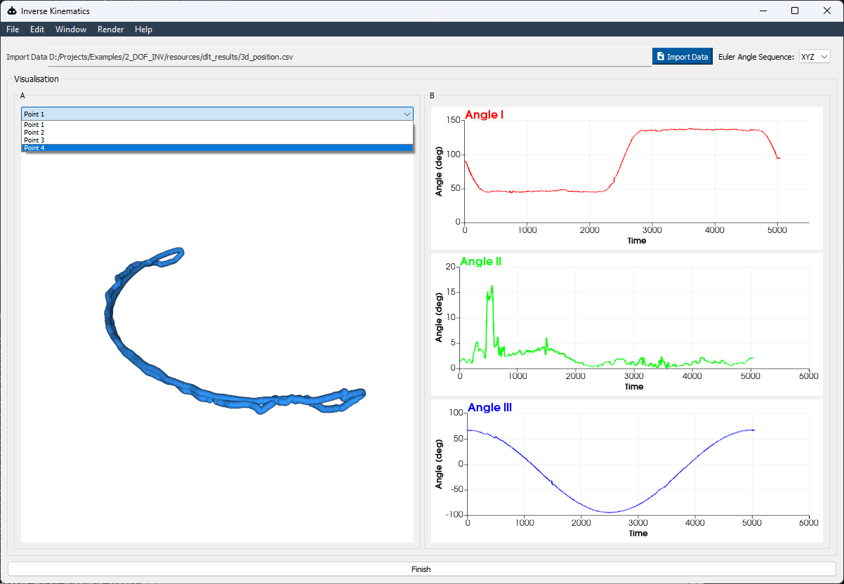
Figure: 3D position data loaded into Inverse kinematics window.

10. Once configuration is complete, click Finish. You’ll return to the Scene Creator Window where the new sprite will appear in green, indicating success.

11. Click Import Scene to finalize the scene. You’ll be redirected back to the Project Creator Window, with the Create Scene button now showing green.

12. Finally, click the Create Project button. This will generate the same project structure and configuration as in the original 2_DOF_INV/ folder provided in project.zip.

References

[1]

Ty Hedrick. DLTdv: A MATLAB-based tool for 2D video digitizing and 3D reconstruction. Available at: https://biomech.web.unc.edu/dltdv/

Download

Get the resource from: Download Link